The Earth Trends Modeler (ETM) is an integrated suite of tools within TerrSet for the analysis of image time series data associated with Earth Observation remotely sensed imagery. With Earth Trends Modeler, users can rapidly assess long term climate trends, measure seasonal trends in phenology, and decompose image time series to seek recurrent patterns in space and time.
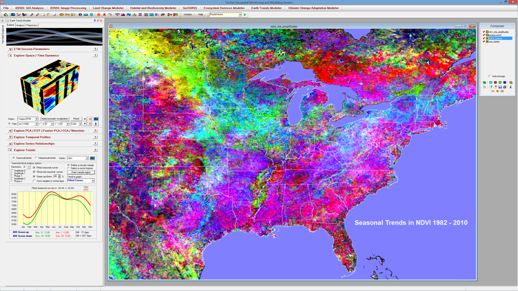
The Earth Trends Modeler (ETM) is specially designed for the analysis of earth observation image time series. In this illustration, a series of 348 global images of monthly NDVI vegetation index data were analyzed for the presence of trends in seasonality. Pixels colored gray (which are almost absent) indicate a stable seasonality. All other colors represent trends. ETM provides an interactive legend (lower left) to interpret the trend for any area (the area in eastern Alabama and western Georgia in this case). The green curve represents the beginning of the series (1982) while the red one represents the end (2010). The X axis is time and the Y axis is NDVI. As can be seen, NDVI has generally increased with a growing bimodality. Spring is coming a bit earlier (11 days) and the autumn is extending longer (almost 30 days).
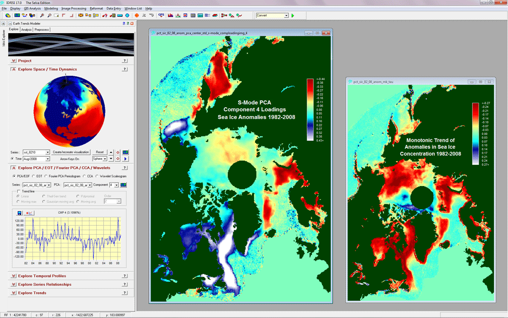
ETM can be used to analyze any kind of image time series. The most common formats are NetCDF and HDF, both of which are directly supported. However, many data are in more idiosyncratic formats. The analyses illustrated here use sea ice concentration data access for free from the U.S. National Snow and Ice Data Center (NSIDC). The documentation on the NSIDC web site indicates that the data are stored as unsigned byte values in flat binary files with a 300 byte header. This is easily imported using IDRISI’s flexible generic raster import routine. The images show part of a Principal Components Analysis as well as a non-linear trend analysis for the period from 1982-2008.
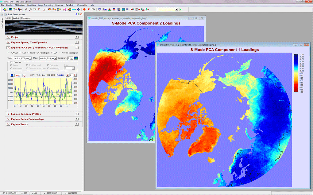
A Principal Components Analysis (PCA) of monthly MODIS Land Surface Temperature (LST) anomalies from 2001 to 2011 for the Arctic region. The first S-mode principal component (foreground) shows a distinctive spatial pattern associated with a rapidly oscillating temporal pattern (the blue line in the graph). To identify it, several well-known climate teleconnection indices were overlaid on the component (the green line on the graph). The overlaid index series uses the secondary axis and ETM also provides the option to invert the Y axis. This was done in this case to show that the first component is clearly the Arctic Oscillation (AO) – a coupled troposphere/stratosphere pressure pattern. Thus the AO can explain the greatest extent of variability in LST over this 10 year period. Note that when comparing index series such as the component and AO index in the graph, the comparison index can be slid back and forth to check for a lagged relationship. ETM indicates the lagged correlation when this is done.
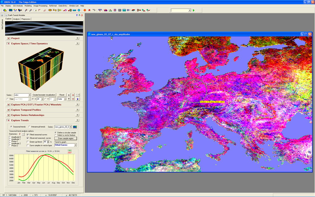
A Seasonal Trend Analysis (STA) of monthly normalized difference vegetation index (NDVI) imagery for Europe from 1982 to 2007. An area of interest in Germany has been circled. The seasonal response graph shows that vegetation productivity has increased throughout the winter and spring, and to a lesser extent in the autumn between the start of the series in 1982 (the green line) versus 2007 (the red line). The graph also shows that spring has advanced by about a month over this period of time. However, the late summer shows a slight decline in productivity.
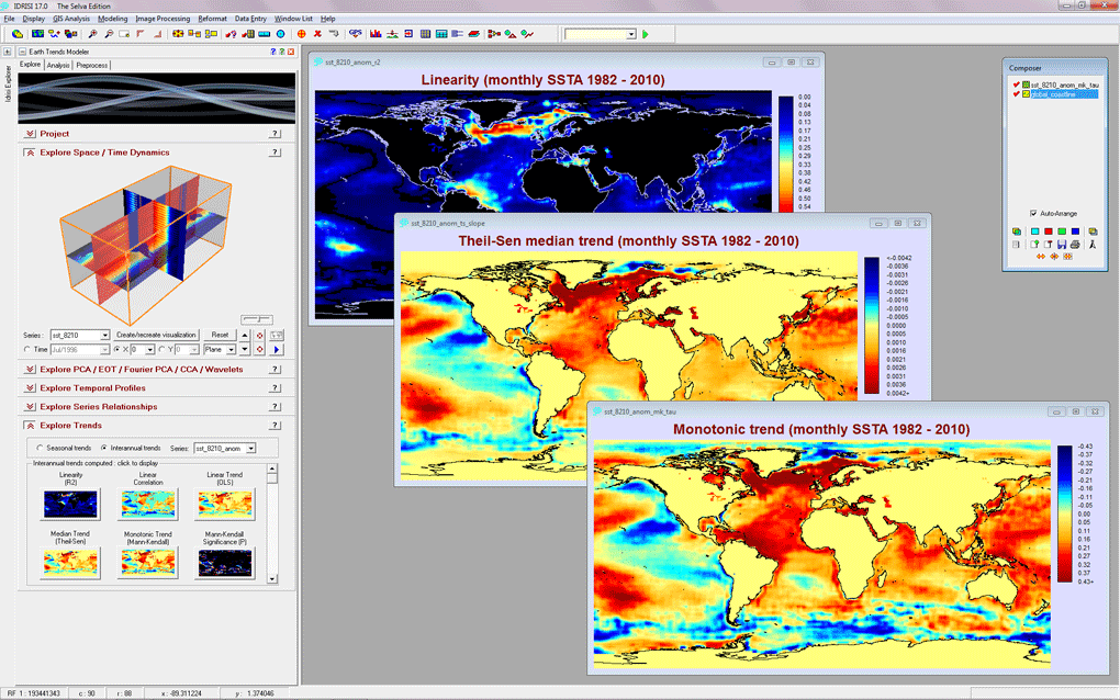
Three of the temporal trend measures provided by ETM. In this case it illustrates an analysis of monthly anomalies in sea surface temperature from 1982 to 2010. The top image expresses the degree to which a linear trend is present. Note that the most linear trends can be found in the north Atlantic sub-polar gyre off of Greenland and at the mouth of the Orinoco river in South America. The middle image is a measure of the rate of change using a special noise-resistant trend measure known as the Theil-Sen median slope. The bottom image expresses trend monotonicity – the degree to which a consistently increasing or decreasing trend can be found (but not necessarily linear).
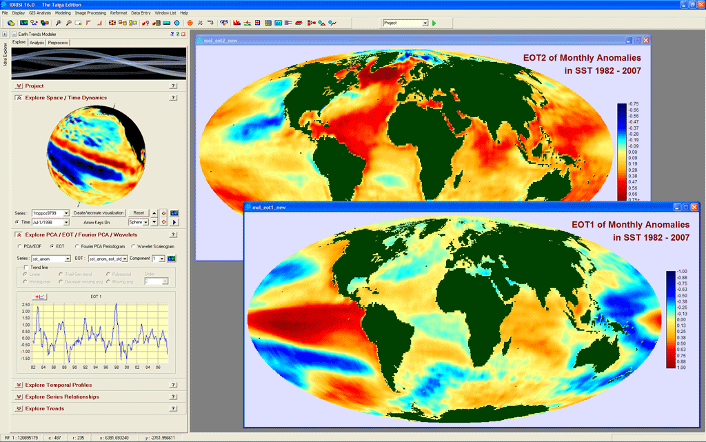
An Empirical Orthogonal Teleconnection (EOT) analysis of monthly anomalies in sea surface temperature (SST) from 1982 to 2007. EOT is a regression-based spectral decomposition technique which is similar in intent and character to an obliquely rotated Principal Components Analysis. Each EOT represents a major pattern of variability over time. The graph shows EOT1 which is clearly the El Niño/Southern Oscillation (ENSO) phenomenon while the foreground image shows what is known as the loading image – the correlation (over time) of each pixel location with this temporal pattern. The background image is the loading image for EOT2 – a combination of the Atlantic Multidecadal Oscillation with a global warming signal.
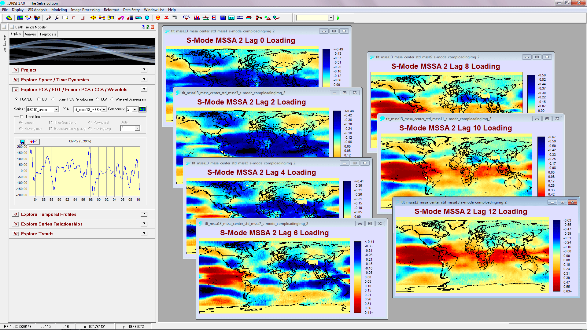
A Multichannel Singular Spectrum Analysis (MSSA) of monthly anomalies in lower tropospheric temperature (1982-2010) using an embedding dimension of 13 months. The embedding dimension establishes a time frame of focus in the analysis of evolving spatio-temporal events, and also indicates that the analysis will be run as an Extended PCA on 13 lagged versions of the same series. In this example, the temporal graph again shows an obvious relationship to El Niño, but instead of a single loading image, this analysis has one for each of the 13 lags (only six are shown). These images are like the frames of a movie loop that show the evolution of the lower tropospheric response to the El Niño/La Niña phenomenon.
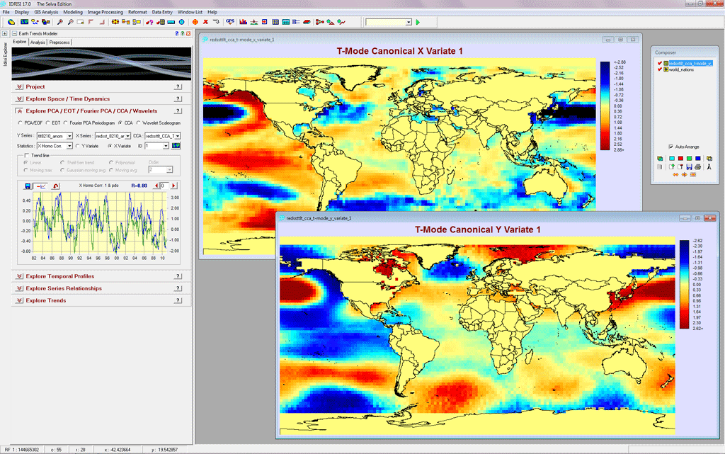
The result of a T-mode Canonical Components Analysis (CCA) of monthly anomalies in sea surface temperature versus monthly anomalies in lower tropospheric temperature from 1982-2010. Traditional S-mode CCA looks for recurrent temporal patterns across the two data series. In T-mode analysis, it is looking for recurrent spatial patterns. In this global analysis, it turns out that the predominant global spatial pattern is that of the Pacific Decadal Oscillation (PDO). In the graph, the index to PDO published by NOAA is plotted (in green) on top of the X-variate (sea-surface temperature) homogenous correlation (in blue). The correlation is 0.80. An equivalent S-mode CCA finds that the familiar ENSO (El Niño Southern Oscillation) pattern is the most prevalent pattern over time.
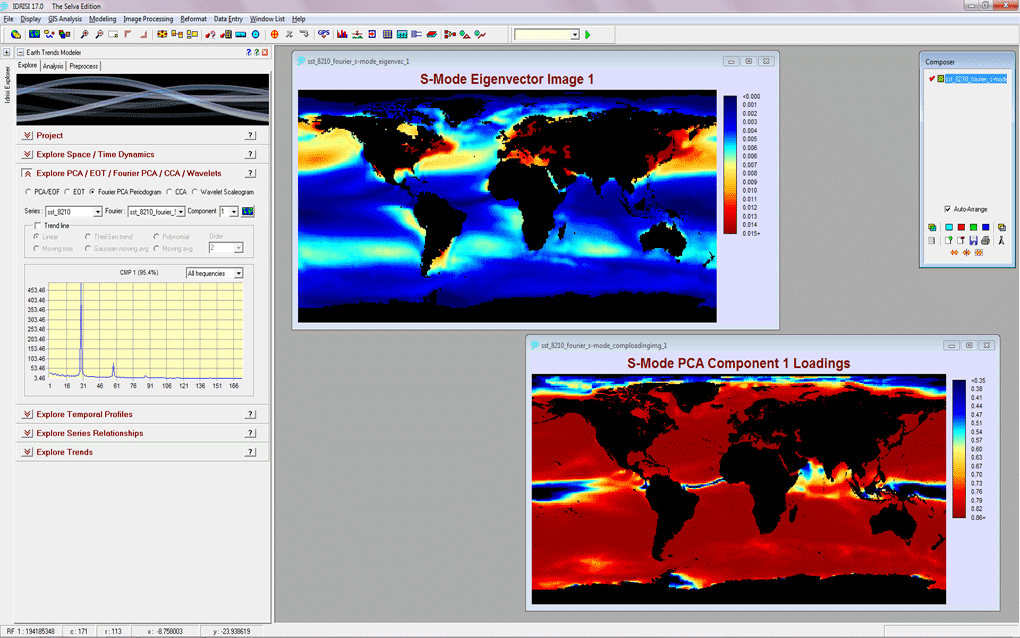
An analysis of monthly sea surface temperature from 1982-2010 using Fourier-PCA. Leading modes of a Fourier-PCA analysis show major patterns of variability that can be described as combinations of sinusoidal waves. The components from this procedure are periodograms with the x-axis representing frequency as wave numbers. This first component shows a strong peak at 29 waves over the 29-year series (with a couple of minor harmonics). It therefore represents the annual cycle. The loading image (lower right) shows that almost all ocean regions (with the exception of the poles and the thermal equator) exhibit prevalent seasonality. However, the eigenvector image shows that the seasonal effect is most extreme in the northern mid-latitudes.
ETM can be used to analyze any kind of image time series. The most common formats are NetCDF and HDF, both of which are directly supported. However, many data are in more idiosyncratic formats. The analyses illustrated here use sea ice concentration data access for free from the U.S. National Snow and Ice Data Center (NSIDC). The documentation on the NSIDC web site indicates that the data are stored as unsigned byte values in flat binary files with a 300 byte header. This is easily imported using IDRISI’s flexible generic raster import routine. The images show part of a Principal Components Analysis as well as a non-linear trend analysis for the period from 1982-2008.
An Empirical Orthogonal Teleconnection (EOT) analysis of monthly anomalies in sea surface temperature (SST) from 1982 to 2007. EOT is a regression-based spectral decomposition technique which is similar in intent and character to an obliquely rotated Principal Components Analysis. Each EOT represents a major pattern of variability over time. The graph shows EOT1 which is clearly the El Niño/Southern Oscillation (ENSO) phenomenon while the foreground image shows what is known as the loading image – the correlation (over time) of each pixel location with this temporal pattern. The background image is the loading image for EOT2 – a combination of the Atlantic Multidecadal Oscillation with a global warming signal.
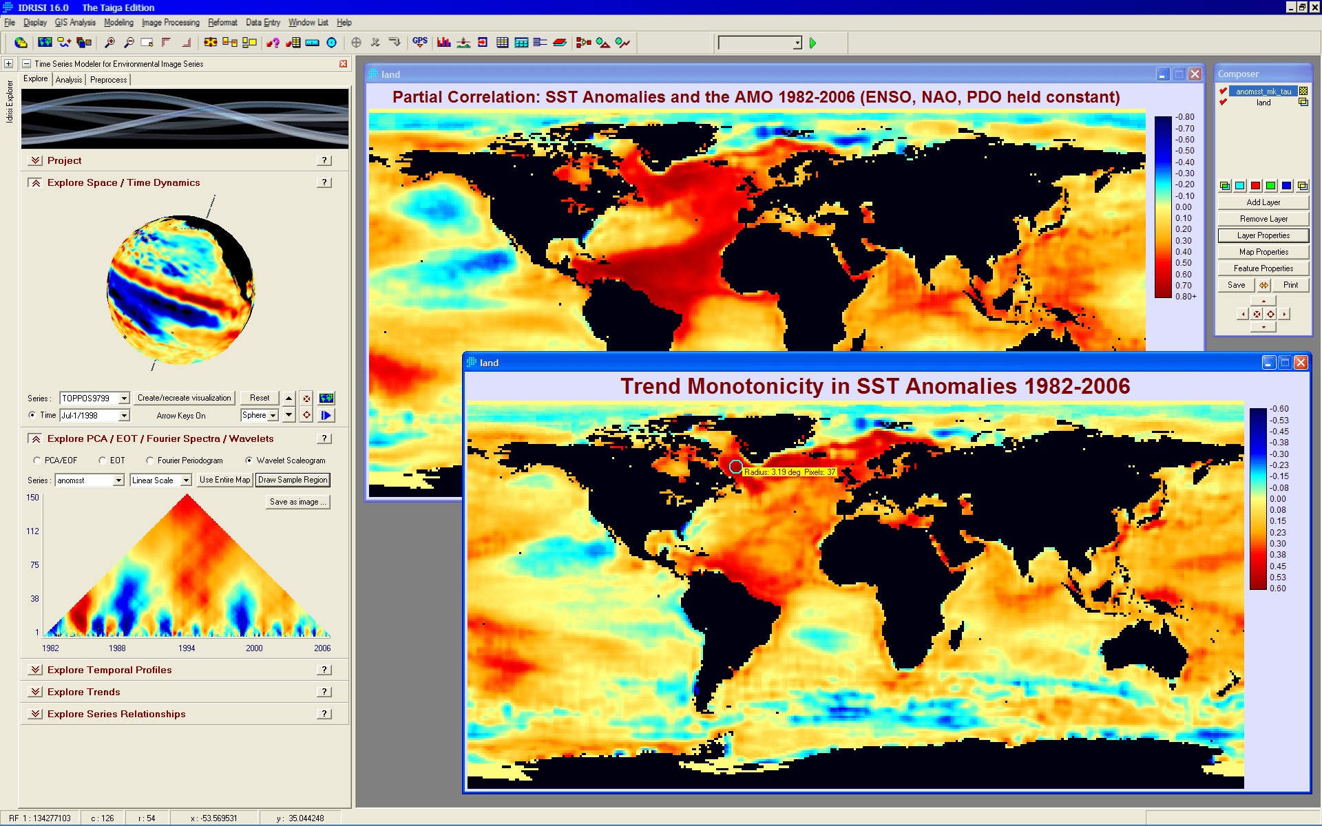
An analysis of trends in sea surface temperature from 1982 to 2006. The strong monotonic trend of increasing temperature in the Atlantic is seen to be related to the Atlantic Multidecadal Oscillation (AMO) as determined from a temporal regression with four major climate teleconnection indices.
With ETM, users can address such questions as:
- “How have temperatures changed over the past 30 years?”
- “Are plants exhibiting a later senescence?”
- “Are there recurrent spatial patterns in phytoplankton productivity?”
- “What are the geographic impacts of climate events such as El Niño?”
No other software technology provides such a coordinated suite of data mining tools needed by the earth system science community for climate change analysis and impact assessment.
Tools in ETM include:
- Parametric and non-parametric trend measures
- Seasonal trend analysis
- Principal Components / Empirical Orthogonal Function analysis (PCA/EOF)
- Extended PCA/EOF for the co-analysis of multiple series (EPCA/EEOF)
- Multichannel Singular Spectrum Analysis (MSSA)
- Empirical Orthogonal Teleconnection (EOT) analysis and extended modes
- Canonical Correlation Analysis (CCA)
- Lagged Linear Modeling
- Fourier PCA and Wavelet analysis
While ETM is intended for professional use, its simple and intuitive interface makes it an excellent tool for teaching and self-exploration. The system includes a full tutorial and sample data sets.
Earth Trends Modeler Key Features
- Extract and analyze long-term global trends and their impacts
- Examine the relationship between time series
- Examine trends in seasonality
- Isolate true change from normal environmental variability
- Uncover and analyze patterns of variability across temporal scales
- Preprocess image time series data including noise removal and deseasoning
Earth Trends Modeler Analytical Features
- Animated 3-D display of space-time cubes
- Dynamic lag correlation between index time series
- Interactive Maximum Overlap Discrete Wavelet analysis
- Trend analysis of index time series (linear trend, Theil-Sen median trend, polynomial (up to 9th order), moving average, Gaussian moving average, moving maximum)
- Interactive temporal profiling
- Image series trend analysis (linear trend, degree of linearity, Theil-Sen median trend, monotonic trend, Mann-Kendall trend significance)
- Seasonal Trend Analysis (STA) including interactive interpretation and trend significance mapping
- Principal Components (PCA) / Empirical Orthogonal Function (EOF) analysis (T-mode and S-mode, standardized/unstandardized and centered/uncentered)
- Extended PCA/EOF (T-mode and S-mode, standardized/unstandardized and centered/uncentered)
- Multichannel Singular Spectrum Analysis (T-mode and S-mode, standardized/unstandardized and centered/uncentered)
- Empirical Orthogonal Teleconnection (EOT) analysis (S-mode, standardized/unstandardized and centered/uncentered)
- Extended EOT (S-mode, standardized/unstandardized and centered/uncentered)
- Cross-EOT (S-mode, standardized/unstandardized and centered/uncentered)
- Multichannel EOT (MEOT) (S-mode, standardized/unstandardized and centered/uncentered)
- Canonical Correlation Analysis (CCA) (T-mode and S-mode, standardized/unstandardized and centered/uncentered)
- Fourier PCA (S-mode, unstandardized, centered)
- Index to Image Series and Image to Image Series Multiple Linear Modeling (slope, intercept, R, R2, Adjusted R2, Partial R) at multiple lags plus residual series creation
- Missing Data Interpolation (harmonic interpolation, spatial interpolation, linear temporal interpolation and climatology)
- Denoising via temporal filtering (mean, Gaussian mean, maximum, cumulative sum, cumulative mean) with any arbitrary filter length
- Denoising via Maximum Value Compositing (MVC).
- Denoising via PCA (T-mode and S-mode)
- Denoising via Inverse Fourier Analysis
- Deseasoning (anomalies, standardized anomalies, temporal filter)
- Series generation (linear, SIN, COS)
- Series editing (lagging, truncation, extension, skip selection, temporal aggregation, spatial subsetting, automatic renaming)
- Serial correlation analysis (Durbin-Watson)
- Detrending (linear or difference series)
- Cochrane-Orcutt transformation
- Trend-preserving prewhitening (Wang and Swail procedure)